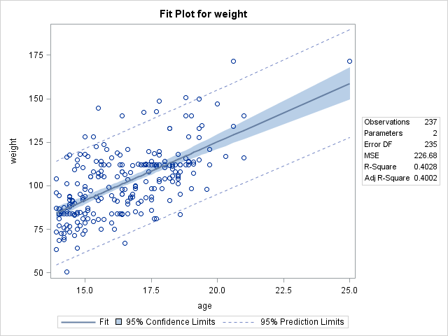
When performing a simple linear regression, it's important to review all the diagnostic plots that come with it. If the residual errors aren't normally distributed, you will have to rethink your model. Like I referenced in an earlier post you can't just stop at the fit plot, even if it is pretty (here courtesy of SAS):

You have to review its diagnostics:

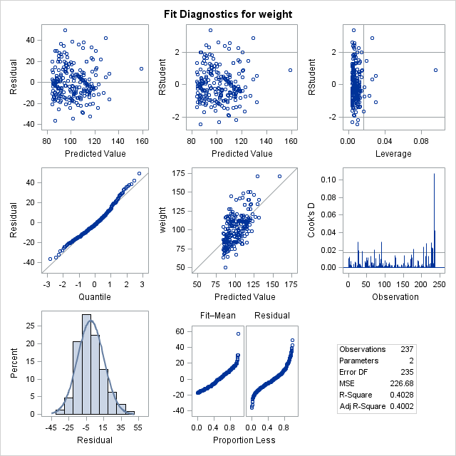
Typically in a set of diagnostic plots like this, you look first at the top left chart to see if the residuals balance around 0. The Q-Q plot below that should be close to the 45° line, the histogram below that should look normal the way most of us know, and the Cook's distance plot at middle right should show no outliers near or above 1. Any of these plots going wrong should be a sign that there's something amiss with your model. And this is all in addition to reviewing the numbers that come out of the model, like the p-value on the F test of the model, the R-square, the p-value on the t test of the dependent variable, and the p-value of a normality test on the residual errors.

The trick is, though, it can take time to develop an intuitive feel for how to read all these numbers and plots, even for a model that's as (relatively) simple as linear regression.

D3.js offers something better, the chance to animate the relationships between these plots, with object constancy. Maybe it would be useful to do something like the transitions in the showreel with the main fit plot and the diagnostic charts, with constancy among the points in the dataset to show which lie where in the various plots I mentioned above from the fit through the diagnostic set. Let's try that.

Simple transitions

The first step is to wrap our heads around the timed transitions in that showreel; I haven't done those before. The key seems to be the use of setTimeout(callback_function, delay) calls at the end of each function in the showreel source. Note that setTimeout() is a JavaScript timer, not a D3 function.

This should be easy to replicate. To try it out, let's just draw a box, then move it around.

This is pretty straightforward, we draw a rect, then we set the first timeout to call one of four similar functions that does what you'd expect:

setTimeout(move_right, duration);

function move_right() {
    test1.select("#box").transition()
        .duration(duration)
        .attr("x", 100);
    setTimeout(move_down, delay + duration);
}

move_right() uses d3's transition() to shift the x over to 100, then sets a time for move_down(), which shifts y to 100, then sets a timeout with a similar callback to move_left(), then we go to move_up(), which goes back to move_right(), and we have an endless loop of timed transitions. This might not be a model for building UI event-driven animations, of course, but we can settle on this kind of showreel-style series of repeating transitions to show a cycle of plots.

Note that the setTimeout delay on each callback isn't just delay but is rather delay + duration. The delay alone runs concurrent with the transition duration, so if we don't add duration, the delay will end at nearly the same time as the duration! The duration means the transition will take duration milliseconds, but javascript still executes the following call to setTimeout immediately, so we have to set the delay value to something longer or the box will never appear to "pause" between transitions.

Adding constancy

The next trick is to do the same thing but with multiple moving points based on data. To do this, we'll expand our model above to include a simple three-value dataset. We'll still move it right, down, left, up, then right again, but in each of these quadrants we'll use a different set of scales to position each element. It's important to use d3's data binding for this rather than, say, a few circle and rect elements we could draw by hand because ultimately we will want to bind real data from a regression.

We'll use the same structure - four functions with obvious names. The first time through, we'll place circles using the straight values as their x and y positions in the upper left quadrant, then for each of the other functions we'll use different scales to slide them around inside each following quadrant. I've added lines to help distinguish the quadrants.

This works pretty well once you are clear about the scope of the object you want to operate on. At first we create a set of svg g group objects, and place circles inside of each:

var g = test2.selectAll("g")
    .data(data)
    .enter().append("g")
    .attr("class", "object");

    g.each(function(d, i) {
        var o = d3.select(this);
            o.append("circle")
            .attr("r", 15)
            .attr("cx", d)
            .attr("cy", d)
            .attr("fill-opacity", ".80")
            .attr("fill", color_scale(i));
    });

This sets us up with the basic set of "data points" we'll move around. Then we just start firing up transitions like before, using setTimeout(), but with each move function doing a little more:

function move_left2() {
    var x = d3.scale.linear()
        .domain([0, 100])
        .range([60, 40]);

    var c = test2.selectAll(".object");
        c.each(function(d, i) {
            var o = d3.select(this);
                o.select("circle").transition()
                    .duration(duration)
                    .attr("cx", x(d))
                    .attr("cy", x(d))
                    .attr("transform", "translate(0, 100)");
        });
    setTimeout(move_up2, delay + duration);
}

First we define a new scale for each quadrant, changing the output range; in this case, it reverses the ordering, and places the circles in a narrow band just 20 pixels wide. Next, we select the .objects we created, which pulls up those gs we started with, then loops through the set of them, firing off a transition the moves the cx and cy of each according to the new scale, and also resets the coordinate space to each quadrant in turn.

Simulating a regression

We'll use a more substantial dataset when we put it all together, but for now let's assemble a small dataset and sketch a fit plot and residual plot transitioning back and forth. I've made up some values and used R to generate a regression (d is just the same data as in the javascript below):

Call:
lm(formula = d ~ seq(0, 10))

Coefficients:
(Intercept)   seq(0, 10)  
     18.000        9.036

We can use this regression line to get a feel for transitioning more elements together, and for some of the extra elements we'll want to add to make things pop a bit.

For the regression, we apply the results R gave us to define the slope, intercept, and a function that returns expected values from the model:

var slope = 9.036;
var intercept = 18;
function expected(index) {
    return (slope * index) + intercept;
    };

This function lets us put in an index number for a data value and get back what the model expects the data value to be. We can then use this whenever we need to plot the residual, here in the original rendering of the data points and residual lines against the model:

g.each(function(d, i) {
    var o = d3.select(this);
    o.attr("class", "observation");
    o.append("line")
        .attr("x1", x(i))
        .attr("y1", y(d))
        .attr("x2", x(i))
        .attr("y2", y(expected(i)))
        .attr("stroke-width", 2)
        .attr("stroke", "gray");
    o.append("circle")
        .attr("r", 5)
        .attr("cx", x(i))
        .attr("cy", y(d))
        .attr("stroke", "black")
        .attr("fill", "darkslategrey");
});

The line is vertical, so the x-scale places it horizontally using the index number. The vertical line segment representing the residual error starts at the actual value d and ends at the expected value expected(i), with both adjusted to the y-scale using y(). Then, in the residual view/function, we just have to rotate the model line to "level" (height/2) and translate the g-wrapped residual line and data point to level minus the y-scale-adjusted expected value from the model:

.attr("transform", "translate(0, " + (200 - y(expected(i))) + ")");

And when we switch back to the "fit" view, we just translate them back again to (0, 0), and rotate the model line back to the original regression slope.

This feels like a good stopping point for today. Next time, we'll pick up from here, add the additional diagnostic plots, and fill out each stage with axes and other niceties as appropriate.